Note
Go to the end to download the full example code.
Imaging example#
How to create visibility from pixel data and make images.
The example uses stixpy to obtain STIX pixel data and convert these into visibilities and xrayvisim
to make the images.
Imports
import logging

import astropy.units as u
import matplotlib.pyplot as plt
import numpy as np
from sunpy.coordinates import HeliographicStonyhurst, Helioprojective
from sunpy.map import Map, make_fitswcs_header
from sunpy.time import TimeRange
from xrayvision.clean import vis_clean
from xrayvision.imaging import vis_to_image, vis_to_map
from xrayvision.mem import mem, resistant_mean

from stixpy.calibration.visibility import calibrate_visibility, create_meta_pixels, create_visibility
from stixpy.coordinates.frames import STIXImaging
from stixpy.coordinates.transforms import get_hpc_info
from stixpy.imaging.em import em
from stixpy.map.stix import STIXMap  # noqa
from stixpy.product import Product

logger = logging.getLogger(__name__)
Read science file as Product
cpd_sci = Product(
    "http://pub099.cs.technik.fhnw.ch/fits/L1/2021/09/23/SCI/solo_L1_stix-sci-xray-cpd_20210923T152015-20210923T152639_V02_2109230030-62447.fits"
)
cpd_sci
Files Downloaded:   0%|          | 0/1 [00:00<?, ?file/s]

solo_L1_stix-sci-xray-cpd_20210923T152015-20210923T152639_V02_2109230030-62447.fits:   0%|          | 0.00/48.4M [00:00<?, ?B/s]

solo_L1_stix-sci-xray-cpd_20210923T152015-20210923T152639_V02_2109230030-62447.fits:   0%|          | 1.02k/48.4M [00:00<7:13:26, 1.86kB/s]

solo_L1_stix-sci-xray-cpd_20210923T152015-20210923T152639_V02_2109230030-62447.fits:   0%|          | 65.8k/48.4M [00:00<06:03, 133kB/s]

solo_L1_stix-sci-xray-cpd_20210923T152015-20210923T152639_V02_2109230030-62447.fits:   0%|          | 211k/48.4M [00:00<01:54, 422kB/s]

solo_L1_stix-sci-xray-cpd_20210923T152015-20210923T152639_V02_2109230030-62447.fits:   1%|          | 598k/48.4M [00:00<00:38, 1.23MB/s]

solo_L1_stix-sci-xray-cpd_20210923T152015-20210923T152639_V02_2109230030-62447.fits:   3%|▎         | 1.28M/48.4M [00:00<00:18, 2.57MB/s]

solo_L1_stix-sci-xray-cpd_20210923T152015-20210923T152639_V02_2109230030-62447.fits:   5%|▌         | 2.65M/48.4M [00:01<00:08, 5.36MB/s]

solo_L1_stix-sci-xray-cpd_20210923T152015-20210923T152639_V02_2109230030-62447.fits:  11%|█         | 5.41M/48.4M [00:01<00:03, 11.1MB/s]

solo_L1_stix-sci-xray-cpd_20210923T152015-20210923T152639_V02_2109230030-62447.fits:  22%|██▏       | 10.7M/48.4M [00:01<00:01, 22.1MB/s]

solo_L1_stix-sci-xray-cpd_20210923T152015-20210923T152639_V02_2109230030-62447.fits:  37%|███▋      | 17.7M/48.4M [00:01<00:00, 35.3MB/s]

solo_L1_stix-sci-xray-cpd_20210923T152015-20210923T152639_V02_2109230030-62447.fits:  51%|█████     | 24.5M/48.4M [00:01<00:00, 44.5MB/s]

solo_L1_stix-sci-xray-cpd_20210923T152015-20210923T152639_V02_2109230030-62447.fits:  65%|██████▍   | 31.2M/48.4M [00:01<00:00, 51.0MB/s]

solo_L1_stix-sci-xray-cpd_20210923T152015-20210923T152639_V02_2109230030-62447.fits:  79%|███████▉  | 38.3M/48.4M [00:01<00:00, 56.6MB/s]

solo_L1_stix-sci-xray-cpd_20210923T152015-20210923T152639_V02_2109230030-62447.fits:  93%|█████████▎| 45.3M/48.4M [00:01<00:00, 60.2MB/s]


Files Downloaded: 100%|██████████| 1/1 [00:02<00:00,  2.46s/file]
Files Downloaded: 100%|██████████| 1/1 [00:02<00:00,  2.46s/file]

CompressedPixelData   <sunpy.time.timerange.TimeRange object at 0x7fa0c70b3610>
    Start: 2021-09-23 15:20:15
    End:   2021-09-23 15:26:39
    Center:2021-09-23 15:23:27
    Duration:0.004439814814814813 days or
           0.10655555555555551 hours or
           6.393333333333331 minutes or
           383.59999999999985 seconds
    DetectorMasks
    [0...697]: [0,1,2,3,4,5,6,7,8,9,10,11,12,13,14,15,16,17,18,19,20,21,22,23,24,25,26,27,28,29,30,31]

    PixelMasks
    [0...697]: [['1' '1' '1' '1' '1' '1' '1' '1' '1' '1' '1' '1']]

    EnergyEdgeMasks
    [0]: [_,1,2,3,4,5,6,7,8,9,10,11,12,13,14,15,16,17,18,19,20,21,22,23,24,25,26,27,28,29,30,31,_]
Read background file as Product
cpd_bkg = Product(
    "http://pub099.cs.technik.fhnw.ch/fits/L1/2021/09/23/SCI/solo_L1_stix-sci-xray-cpd_20210923T095923-20210923T113523_V02_2109230083-57078.fits"
)
cpd_bkg
Files Downloaded:   0%|          | 0/1 [00:00<?, ?file/s]

solo_L1_stix-sci-xray-cpd_20210923T095923-20210923T113523_V02_2109230083-57078.fits:   0%|          | 0.00/121k [00:00<?, ?B/s]

solo_L1_stix-sci-xray-cpd_20210923T095923-20210923T113523_V02_2109230083-57078.fits:   1%|          | 1.02k/121k [00:00<01:04, 1.86kB/s]

solo_L1_stix-sci-xray-cpd_20210923T095923-20210923T113523_V02_2109230083-57078.fits:  47%|████▋     | 57.2k/121k [00:00<00:00, 117kB/s]


Files Downloaded: 100%|██████████| 1/1 [00:01<00:00,  1.26s/file]
Files Downloaded: 100%|██████████| 1/1 [00:01<00:00,  1.26s/file]

CompressedPixelData   <sunpy.time.timerange.TimeRange object at 0x7fa0c719a490>
    Start: 2021-09-23 09:59:23
    End:   2021-09-23 11:35:23
    Center:2021-09-23 10:47:23
    Duration:0.06666666666666665 days or
           1.5999999999999996 hours or
           95.99999999999997 minutes or
           5759.999999999999 seconds
    DetectorMasks
    [0]: [0,1,2,3,4,5,6,7,8,9,10,11,12,13,14,15,16,17,18,19,20,21,22,23,24,25,26,27,28,29,30,31]

    PixelMasks
    [0]: [['1' '1' '1' '1' '1' '1' '1' '1' '1' '1' '1' '1']]

    EnergyEdgeMasks
    [0]: [_,1,2,3,4,5,6,7,8,9,10,11,12,13,14,15,16,17,18,19,20,21,22,23,24,25,26,27,28,29,30,31,32]
Set time and energy ranges which will be considered for the science and the background file
time_range_sci = ["2021-09-23T15:21:00", "2021-09-23T15:24:00"]
time_range_bkg = [
    "2021-09-23T09:00:00",
    "2021-09-23T12:00:00",
]  # Set this range larger than the actual observation time
energy_range = [28, 40] * u.keV
Create the meta pixel, A, B, C, D for the science and the background data
meta_pixels_sci = create_meta_pixels(
    cpd_sci, time_range=time_range_sci, energy_range=energy_range, flare_location=[0, 0] * u.arcsec, no_shadowing=True
)

meta_pixels_bkg = create_meta_pixels(
    cpd_bkg, time_range=time_range_bkg, energy_range=energy_range, flare_location=[0, 0] * u.arcsec, no_shadowing=True
)
Perform background subtraction
meta_pixels_bkg_subtracted = {
    **meta_pixels_sci,
    "abcd_rate_kev_cm": meta_pixels_sci["abcd_rate_kev_cm"] - meta_pixels_bkg["abcd_rate_kev_cm"],
    "abcd_rate_error_kev_cm": np.sqrt(
        meta_pixels_sci["abcd_rate_error_kev_cm"] ** 2 + meta_pixels_bkg["abcd_rate_error_kev_cm"] ** 2
    ),
}
Create visibilities from the meta pixels
vis = create_visibility(meta_pixels_bkg_subtracted)
Calibrate the visibilities
cal_vis = calibrate_visibility(vis)
Selected detectors 10 to 7
# order by sub-collimator e.g. 10a, 10b, 10c, 9a, 9b, 9c ....
isc_10_7 = [3, 20, 22, 16, 14, 32, 21, 26, 4, 24, 8, 28]
idx = np.argwhere(np.isin(cal_vis.meta["isc"], isc_10_7)).ravel()
Slice the visibilities to detectors 10 - 7
vis10_7 = cal_vis[idx]
Set up image parameters
imsize = [512, 512] * u.pixel  # number of pixels of the map to reconstruct
pixel = [10, 10] * u.arcsec / u.pixel  # pixel size in arcsec
Make a full disk back projection (inverse transform) map
bp_image = vis_to_image(vis10_7, imsize, pixel_size=pixel)
Obtain the necessary metadata to create a sunpy map in the STIXImaging frame
vis_tr = TimeRange(vis.meta["time_range"])
roll, solo_xyz, pointing = get_hpc_info(vis_tr.start, vis_tr.end)
solo = HeliographicStonyhurst(*solo_xyz, obstime=vis_tr.center, representation_type="cartesian")
coord = STIXImaging(0 * u.arcsec, 0 * u.arcsec, obstime=vis_tr.start, obstime_end=vis_tr.end, observer=solo)
header = make_fitswcs_header(
    bp_image, coord, telescope="STIX", observatory="Solar Orbiter", scale=[10, 10] * u.arcsec / u.pix
)
fd_bp_map = Map((bp_image, header))
Files Downloaded:   0%|          | 0/1 [00:00<?, ?file/s]

solo_L2_stix-aux-ephemeris_20210923_V02U.fits:   0%|          | 0.00/397k [00:00<?, ?B/s]

solo_L2_stix-aux-ephemeris_20210923_V02U.fits:   0%|          | 1.02k/397k [00:00<02:09, 3.06kB/s]

solo_L2_stix-aux-ephemeris_20210923_V02U.fits:   8%|▊         | 33.0k/397k [00:00<00:03, 96.7kB/s]

solo_L2_stix-aux-ephemeris_20210923_V02U.fits:  43%|████▎     | 170k/397k [00:00<00:00, 463kB/s]


Files Downloaded: 100%|██████████| 1/1 [00:00<00:00,  1.10file/s]
Files Downloaded: 100%|██████████| 1/1 [00:00<00:00,  1.10file/s]
Convert the coordinates and make a map in Helioprojective and rotate so “North” is “up”
hpc_ref = coord.transform_to(Helioprojective(observer=solo, obstime=vis_tr.center))  # Center of STIX pointing in HPC
header_hp = make_fitswcs_header(bp_image, hpc_ref, scale=[10, 10] * u.arcsec / u.pix, rotation_angle=90 * u.deg + roll)
hp_map = Map((bp_image, header_hp))
hp_map_rotated = hp_map.rotate()
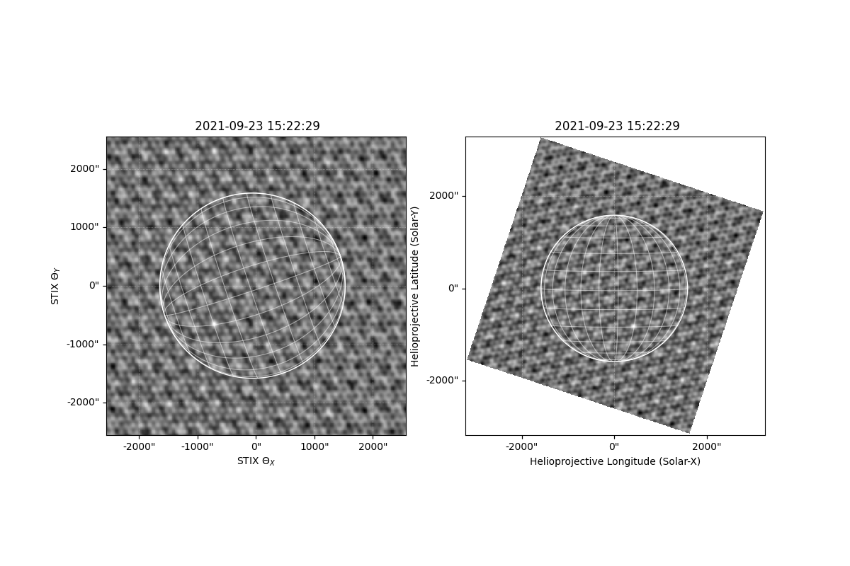
Plot the both maps
fig = plt.figure(figsize=(12, 8))
ax0 = fig.add_subplot(1, 2, 1, projection=fd_bp_map)
ax1 = fig.add_subplot(1, 2, 2, projection=hp_map_rotated)
fd_bp_map.plot(axes=ax0)
fd_bp_map.draw_limb()
fd_bp_map.draw_grid()

hp_map_rotated.plot(axes=ax1)
hp_map_rotated.draw_limb()
hp_map_rotated.draw_grid()
Files Downloaded:   0%|          | 0/1 [00:00<?, ?file/s]
Files Downloaded: 100%|██████████| 1/1 [00:00<00:00,  3.04file/s]
Files Downloaded: 100%|██████████| 1/1 [00:00<00:00,  3.04file/s]

<CoordinatesMap with 2 world coordinates:

  index aliases    type   unit    wrap   format_unit visible
  ----- ------- --------- ---- --------- ----------- -------
      0     lon longitude  deg 180.0 deg         deg     yes
      1     lat  latitude  deg      None         deg     yes

>
Estimate the flare location and plot on top of back projection map. Note the coordinates are automatically converted from the STIXImaging to Helioprojective
max_pixel = np.argwhere(fd_bp_map.data == fd_bp_map.data.max()).ravel() * u.pixel
# because WCS axes and array are reversed
max_stix = fd_bp_map.pixel_to_world(max_pixel[1], max_pixel[0])

ax0.plot_coord(max_stix, marker=".", markersize=50, fillstyle="none", color="r", markeredgewidth=2)
ax1.plot_coord(max_stix, marker=".", markersize=50, fillstyle="none", color="r", markeredgewidth=2)
[<matplotlib.lines.Line2D object at 0x7fa0c3477190>]
Use estimated flare location to create more accurate visibilities
meta_pixels_sci = create_meta_pixels(
    cpd_sci, time_range=time_range_sci, energy_range=energy_range, flare_location=max_stix, no_shadowing=True
)

meta_pixels_bkg_subtracted = {
    **meta_pixels_sci,
    "abcd_rate_kev_cm": meta_pixels_sci["abcd_rate_kev_cm"] - meta_pixels_bkg["abcd_rate_kev_cm"],
    "abcd_rate_error_kev_cm": np.sqrt(
        meta_pixels_sci["abcd_rate_error_kev_cm"] ** 2 + meta_pixels_bkg["abcd_rate_error_kev_cm"] ** 2
    ),
}

vis = create_visibility(meta_pixels_bkg_subtracted)
cal_vis = calibrate_visibility(vis, flare_location=max_stix)
Selected detectors 10 to 3 order by sub-collimator e.g. 10a, 10b, 10c, 9a, 9b, 9c ….
isc_10_3 = [3, 20, 22, 16, 14, 32, 21, 26, 4, 24, 8, 28, 15, 27, 31, 6, 30, 2, 25, 5, 23, 7, 29, 1]
idx = np.argwhere(np.isin(cal_vis.meta["isc"], isc_10_3)).ravel()
Create an xrayvsion visibility object
cal_vis.meta["offset"] = max_stix
vis10_3 = cal_vis[idx]
Set up image parameters
imsize = [129, 129] * u.pixel  # number of pixels of the map to reconstruct
pixel = [2, 2] * u.arcsec / u.pixel  # pixel size in arcsec
Create a back projection image with natural weighting
bp_nat = vis_to_image(vis10_3, imsize, pixel_size=pixel)
Create a back projection image with uniform weighting
bp_uni = vis_to_image(vis10_3, imsize, pixel_size=pixel, scheme="uniform")
Create a sunpy.map.Map with back projection
bp_map = vis_to_map(vis10_3, imsize, pixel_size=pixel)
Crete a clean image using the clean algorithm vis_clean
niter = 200  # number of iterations
gain = 0.1  # gain used in each clean iteration
beam_width = 20.0 * u.arcsec
clean_map, model_map, resid_map = vis_clean(
    vis10_3, imsize, pixel_size=pixel, gain=gain, niter=niter, clean_beam_width=20 * u.arcsec
)
2024-07-16T20:41:52Z INFO xrayvision.clean 124: Iter: 0, strength: 0.7704811709722035, location: (62, 65)
2024-07-16T20:41:52Z INFO xrayvision.clean 124: Iter: 25, strength: 0.17685250348061884, location: (81, 53)
2024-07-16T20:41:52Z INFO xrayvision.clean 124: Iter: 50, strength: 0.08367161699156966, location: (63, 87)
2024-07-16T20:41:52Z INFO xrayvision.clean 145: Largest residual negative
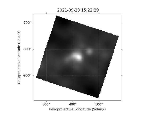
Create a sunpy map for the clean image in Helioprojective
header = make_fitswcs_header(
    clean_map.data,
    max_stix.transform_to(Helioprojective(obstime=vis_tr.center, observer=solo)),
    telescope="STIX",
    observatory="Solar Orbiter",
    scale=pixel,
    rotation_angle=90 * u.deg + roll,
)

clean_map = Map((clean_map.data, header))
plt.figure()
clean_map.rotate().plot()
<matplotlib.image.AxesImage object at 0x7fa0c33e1f10>
Crete a map using the MEM GE algorithm mem
snr_value, _ = resistant_mean((np.abs(vis10_3.visibilities) / vis10_3.amplitude_uncertainty).flatten(), 3)
percent_lambda = 2 / (snr_value**2 + 90)
mem_map = mem(vis10_3, shape=imsize, pixel_size=pixel, percent_lambda=percent_lambda)
2024-07-16T20:41:57Z INFO xrayvision.mem 159: Iter: 0, Chi2: 127.93058284978744
2024-07-16T20:41:57Z INFO xrayvision.mem 159: Iter: 25, Chi2: 4.301970597826388
2024-07-16T20:41:57Z INFO xrayvision.mem 159: Iter: 50, Chi2: 3.186769018989274
2024-07-16T20:41:57Z INFO xrayvision.mem 159: Iter: 75, Chi2: 2.7423076128838018
2024-07-16T20:41:57Z INFO xrayvision.mem 159: Iter: 100, Chi2: 2.4836161402644343
2024-07-16T20:41:57Z INFO xrayvision.mem 159: Iter: 125, Chi2: 2.3153980537684267
2024-07-16T20:41:57Z INFO xrayvision.mem 159: Iter: 150, Chi2: 2.1994253828533328
2024-07-16T20:41:57Z INFO xrayvision.mem 159: Iter: 175, Chi2: 2.113899821452196
/home/docs/checkouts/readthedocs.org/user_builds/stixpy/envs/v0.1.3/lib/python3.9/site-packages/astropy/units/quantity.py:1326: ComplexWarning: Casting complex values to real discards the imaginary part
  self.view(np.ndarray).__setitem__(i, self._to_own_unit(value))
2024-07-16T20:41:58Z INFO xrayvision.mem 510: Iter: 0, Obj function: (139.23212126829804+0j)
2024-07-16T20:42:02Z INFO xrayvision.mem 510: Iter: 25, Obj function: (5.1902301519118135+0j)
2024-07-16T20:42:06Z INFO xrayvision.mem 510: Iter: 50, Obj function: (4.826163622350658+0j)
2024-07-16T20:42:09Z INFO xrayvision.mem 510: Iter: 75, Obj function: (4.7990102763476346+0j)
2024-07-16T20:42:13Z INFO xrayvision.mem 510: Iter: 100, Obj function: (4.794721317122828+0j)
Crete a map using the EM algorithm EM
em_map = em(
    meta_pixels_bkg_subtracted["abcd_rate_kev_cm"],
    cal_vis,
    shape=imsize,
    pixel_size=pixel,
    flare_location=max_stix,
    idx=idx,
)

vmax = max([clean_map.data.max(), mem_map.data.max(), em_map.value.max()])
2024-07-16T20:42:15Z INFO stixpy.imaging.em 180: Iteration: 25, StdDeV: 0.05210401842903427, C-stat: 0.0322101423828504
2024-07-16T20:42:15Z INFO stixpy.imaging.em 180: Iteration: 50, StdDeV: 0.01550496359088871, C-stat: 0.02113078919193867
2024-07-16T20:42:15Z INFO stixpy.imaging.em 180: Iteration: 75, StdDeV: 0.002796184328660909, C-stat: 0.017429889982876513
2024-07-16T20:42:15Z INFO stixpy.imaging.em 180: Iteration: 100, StdDeV: 0.0005577500813556657, C-stat: 0.016355800816783846
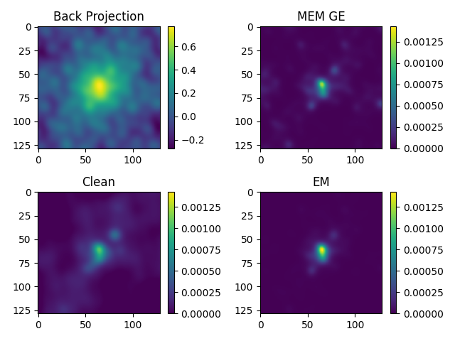
Finally compare the images from each algorithm
fig, axes = plt.subplots(2, 2)
a = axes[0, 0].imshow(bp_nat.value)
axes[0, 0].set_title("Back Projection")
fig.colorbar(a)
b = axes[1, 0].imshow(clean_map.data, vmin=0, vmax=vmax)
axes[1, 0].set_title("Clean")
fig.colorbar(b)
c = axes[0, 1].imshow(mem_map.data, vmin=0, vmax=vmax)
axes[0, 1].set_title("MEM GE")
fig.colorbar(c)
d = axes[1, 1].imshow(em_map.value, vmin=0, vmax=vmax)
axes[1, 1].set_title("EM")
fig.colorbar(d)
fig.tight_layout()
plt.show()
Total running time of the script: (0 minutes 35.766 seconds)